A simulated fault target has engineering value only when it maps to physical behavior. Calibration is not tuning RTL parameters until a fault “looks successful”; it compares target, window, effect, repeatability, and residual mismatch against traceable measurements.
From instrument readings to logic effects
A clinical thermometer needs comparison against a traceable standard; smooth readings do not prove accuracy. Voltage/clock glitches, laser, or EM injection likewise require instrument settings, probe/location, voltage/temperature, trigger timing, chip revision, and repeats. The analogy motivates traceability; it does not claim any injection method necessarily causes a particular RTL flip.
Classify physical outcomes as invalidated, reset, skipped, delayed, corrupted data, checker alert, permanent damage, or no observed effect. Map them conditionally to the digital model: under settings X, location Y, and window Z, estimate the frequency and interval for each effect. One successful attempt does not imply a deterministic bit flip.
Place measurements and models in a layered table: physical stimulus, observable chip response, netlist effect, RTL abstraction. Report sample count, misses, non-repeatability, spatial resolution, and confidence intervals. If the setup sees only reset and not internal nodes, mark that observability limit; do not infer an internal state change.
Separate calibration and validation sets. Estimate the model on one set and check predictive coverage on independent windows; stratify by chip, lot, environment, and revision. Do not extrapolate to untested locations or tools. The interactive lab uses synthetic samples only; it reads no physical measurements and performs no fault injection.
Find model mismatch
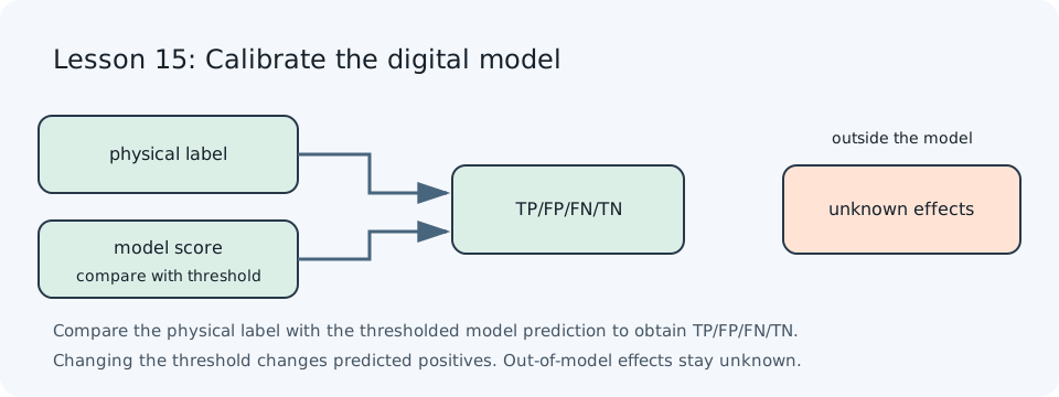
Compare physical outcomes with model predictions using a confusion matrix, especially false negatives: effects seen physically but absent from the model. Version and hash every revision, then rerun the campaign. Conclusions cover only the calibration domain; few samples or zero observations do not make an event impossible.
Offline interactive lab
RTL / SVA review direction
Physical-injection calibration compares measured outcomes with model predictions. An RTL assertion cannot replace that physical evidence.
Check your reasoning
- Recognition — What does a false negative mean during model calibration? Reasoning: Physical injection produced an effect that the digital model did not predict. This gap can hide an acceptance path.
- Contrast — As a score threshold rises, which predictions can change? Reasoning: Predicted positives can stay the same or decrease; they cannot increase. True positives or false positives may fall, while false negatives or true negatives may rise.
- Scenario — The chip shows a multi-bit upset absent from the model. How should it be recorded? Reasoning: Record an out-of-model effect and its physical context. Do not count it as a model negative or silently omit it from the unknowns.
- Failure diagnosis — A report shows zero unknown effects after its unknown list was hidden. What is wrong? Reasoning: Hiding a list does not remove the unknowns. Keep their count and status visible; do not present unobserved or omitted as absent.
- Design risk / transfer — You tune a model on one board and test the same records. What does this establish? Reasoning: It measures fit to that calibration set, not generalization. Hold out physical samples and state the device, setup, conditions, and limits.
References
Laser fault-model RTL/layout validation · SYNFI pre-silicon fault analysis
MY ACADEMY · LESSON FILM
Lesson video
The film explains this lesson’s data path. After a section, return to the interactive exercise and change the input or fault conditions. The animation presents a teaching model; it does not replace RTL simulation.
Swipe the film horizontally, or use the arrow keys to inspect the diagrams.
Diagram scope
Teaching model · Not RTL simulation or silicon testing
Concept / synthetic teaching diagram; not measurement, a certain bit flip or generalization proof
Narration uses a synthetic voice. Both the interaction and animation have model boundaries; interpret results using this lesson’s sources and validation scope.
Wrap-up: take this lesson into a design review
- Threat model and assumptions
A physical campaign records traceable stimulus and chip response; digital targets/effects are calibration hypotheses.
- Why the design fails
One hit is treated as a deterministic bit flip, or an internal register change is inferred without observing it.
- Defenses
Map effects by layer, retain misses and unknowns, validate predictions on separate data, and report intervals.
- Validation and checks to perform
Report sample/location/timing/environment/revision/instrument settings, confusion matrix, and model hash; conclusions cover the calibrated domain only.
- Limits and unverified claims
Small samples, hidden internal nodes, other dies/packages/tools, analog coupling, and unmodeled faults limit extrapolation.
Try a changed assumption
Take one out-of-model effect. Define a new test stratum and the sensing/samples needed before adding it.
This wrap-up summarizes the lesson’s teaching cases, references and experiment scope. Checks not reported as completed remain future work.