Ten plates on hardwired inference
Large-model inference spends time and energy moving weights, not only multiplying them. A GPU often fetches parameters again for the next token. Taalas takes the hard road: fix one model's weights and dataflow into silicon so you move less and repeat less.
The ten plates are a teaching abstraction, not a reverse-engineered HC1 schematic. For one activation x and many low-bit fixed weights, prepare a finite candidate set and let each weight code pick a route. Pictures give intuition; the prose maps each claim to a mechanism, a limit, and what the sources do not support.
Start with reuse. Then look at the bill: wiring, precision, tape-out, and what happens when the model changes.
The model is not loaded; it is built into the chip
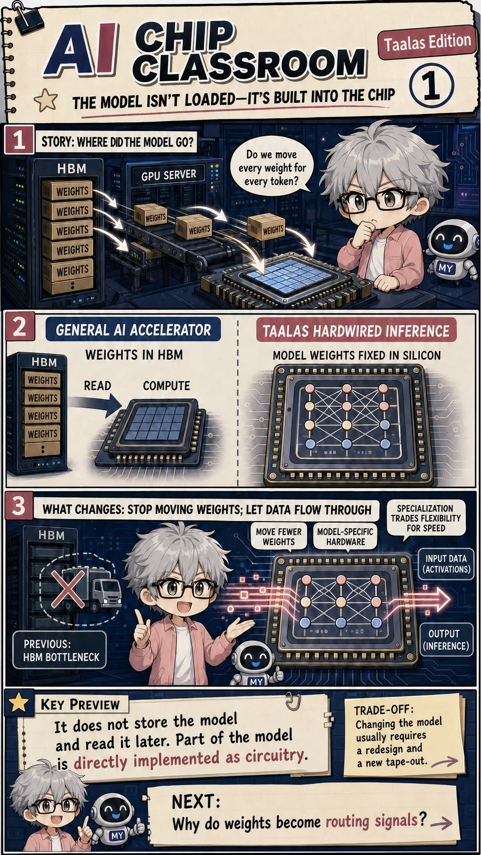
On the left, a stack of HBM crates labelled weights; on the right, a GPU server that has to fetch another crate every time it emits a token. The point is not that GPUs cannot multiply. It is that decode keeps paying the cost of moving the same parameters again.
A conventional accelerator keeps weights in HBM, reads them, then computes. The hardwired side draws those weights into the die, so activations enter on one edge and results leave on the other. The plate crosses out the HBM truck and summarizes three claims: move fewer weights, build model-specific hardware, and let speed come from that specialization.
"Built into the chip" is easy to over-read. It does not mean burning a file, and it does not mean storing an ordinary checkpoint in ROM and reading it the usual way. The model structure and the fixed weights take part in the physical implementation, so the data path can be cut for that model.
Taalas describes this stance as total specialization: one chip serves one model, with storage and computation tightly integrated. For the HC1 demonstrator, the company also says the system does not rely on HBM, advanced packaging, 3D stacking, or liquid cooling. Treat that as a vendor description of this system, not a law of physics for every hardwired design. [1]
Flexibility is the price of that efficiency. A general accelerator can load another model. Changing hardwired base weights or model structure can require redesign and fabrication. Taalas also lists configurable context windows and LoRA support, so those features must be distinguished from replacing the entire base model.
Weights just changed jobs
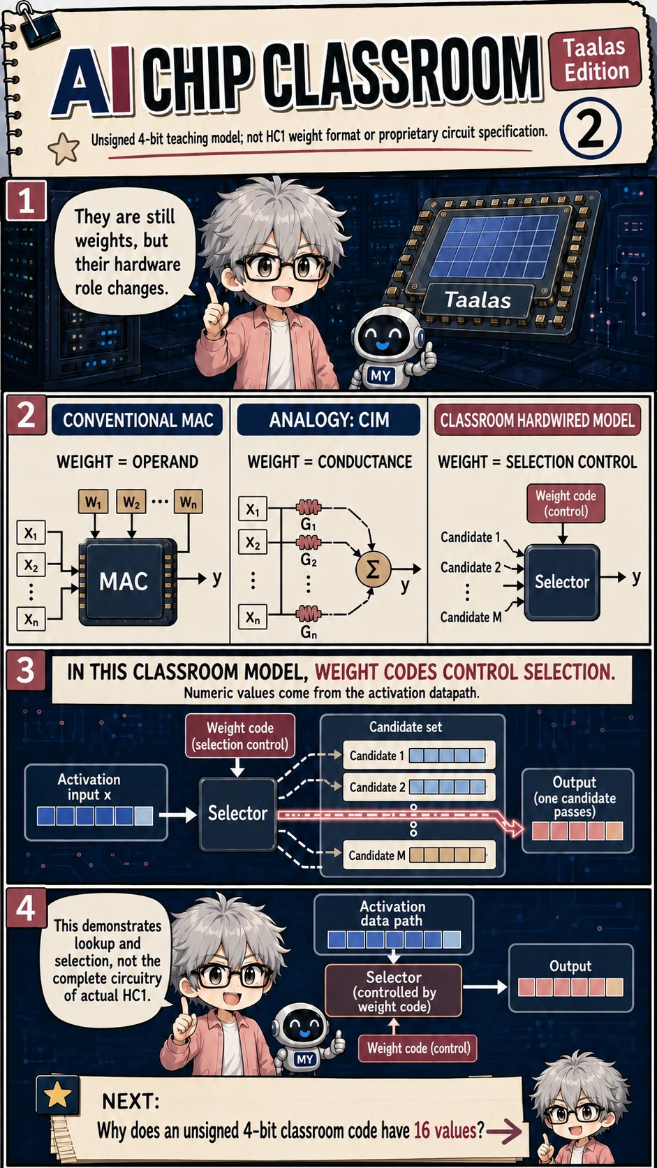
Same word, three jobs. In a conventional MAC, the weight is an operand: multiply with x, then accumulate. In analog compute-in-memory, a weight is often mapped to device conductance, and voltage and current do the multiply-accumulate. In this teaching model, a low-bit weight is an index. Candidates exist first; the weight code picks one.
The selector panel makes the split visible. Activation x enters from the left, the weight code is control, the candidate set sits in the middle, and only one candidate is allowed through. Do not rush to say there is no multiply — numeric values still come from the activation data path. The selector does not invent the answer; it only opens a route.
This is a teaching model, not a transistor-level HC1 schematic. Taalas’s current official account describes a custom three-bit base format and mixed three-/six-bit parameters for its first Silicon Llama; its second generation adopts standard four-bit floating-point formats. Our unsigned four-bit, sixteen-candidate model establishes a functional relationship, not HC1’s parameter format, transistor count or netlist. [3]
The analog-CIM column is the conductance picture. Digital CIM also exists, with bits in memory and arithmetic at the periphery. If you later see the phrase select-in-memory, compute-in-periphery, that is this article's analogy, not an industry taxonomy.
In this model the weight behaves more like routing control than like a value that grows its own product. The next plate shows why four bits suddenly make the candidate set small enough to reuse.
Four bits leave sixteen candidate codes
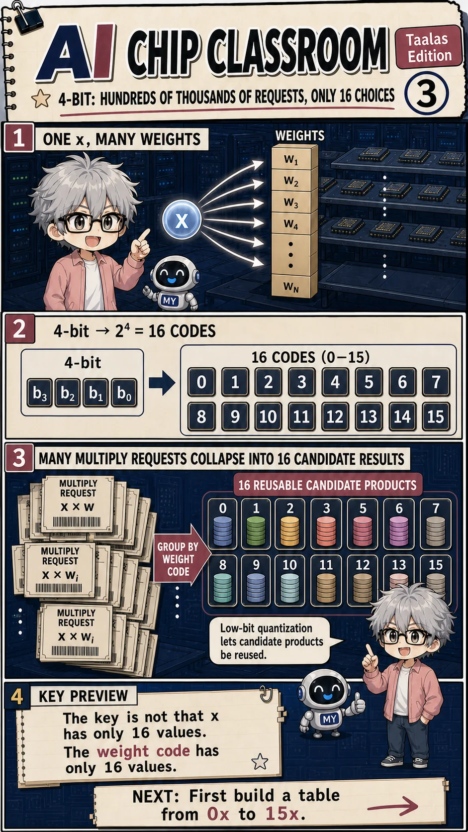
One activation x facing a stack of weights w1 through wn is the shape of a matrix-vector slice. Four bits encode 2^4 = 16 values, drawn as 0 through 15.
The turn is the collapse of multiply tickets into sixteen reusable candidate products. The plate title says ~150,000 requests, only 16 candidates — classroom scale for "a lot," not a published layer size from Taalas. Low-bit quantization matters here: however many weights there are, the index still lands in those sixteen slots.
The correction in large type is worth keeping: the point is not that x has only sixteen values. The point is that the weight code has only sixteen values. For one x, hardware can prepare the candidate products and let many fixed weights select from them. The size of the reusable set is set by weight bit-width, not by the numeric range of the activation.
Real quantized models may be signed, scaled, grouped, or nonuniform. Unsigned 0–15 is the clean teaching grid. Do not copy it out as a product format.
4-bit quantization splits two different questions: how many multiplies you need, versus how many distinct answers you must prepare. The first can be huge; the second is locked by bit-width.
Build the candidate table, then look it up
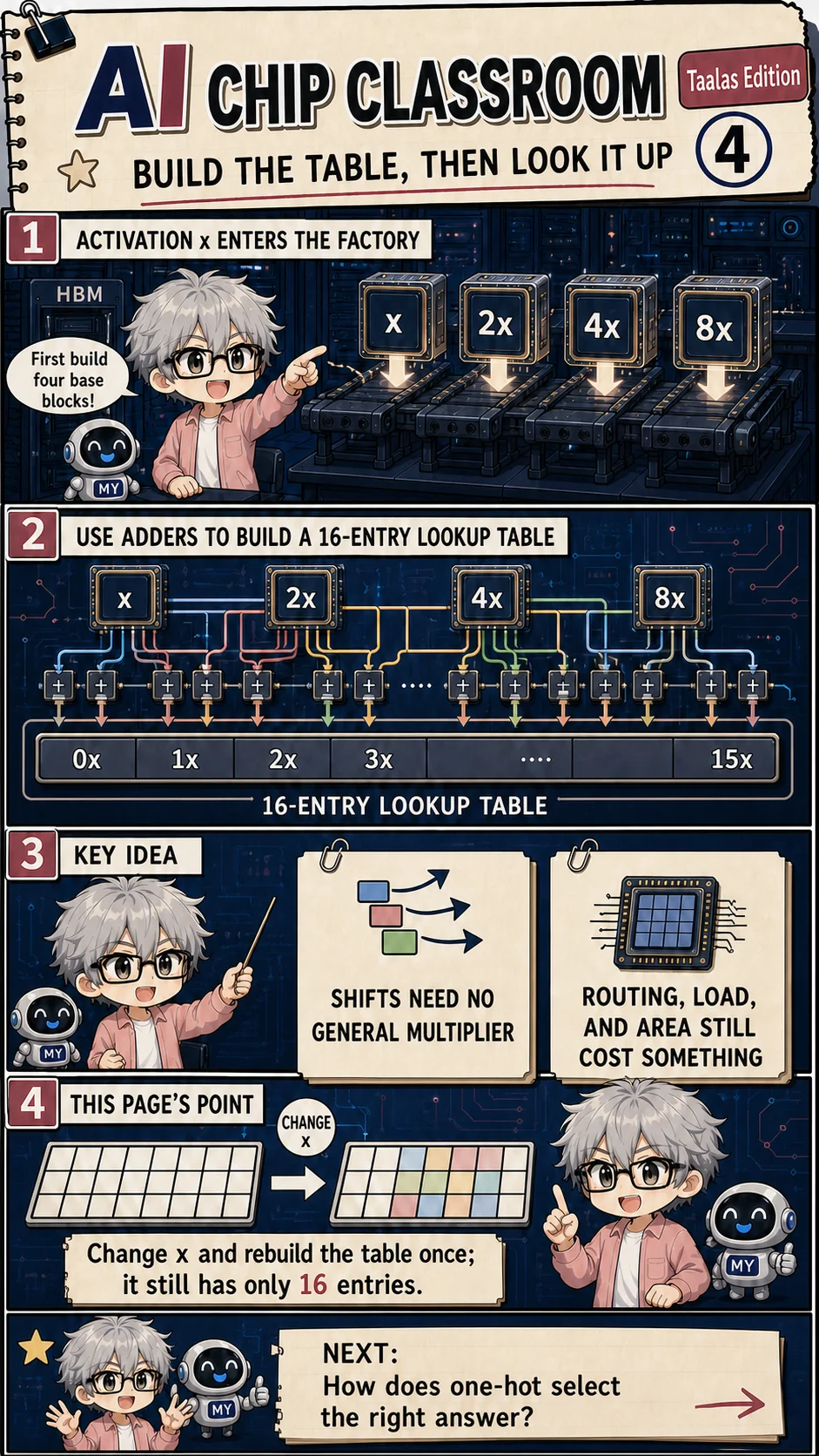
Start with four bases: x, 2x, 4x, and 8x. A left shift is a multiply by two, so those three doubles do not each need a general multiplier. Adders then combine them into 0x through 15x — 6x is 4x plus 2x; 15x is all four bases added. Once the table exists, many fixed weights can share it.
A shift avoids a general multiplier. Wiring, load, area, and timing are still real. "Free" is a nickname that teaches the wrong habit. What you save is repeating a full multiply for every weight. What you still pay is generating candidates and delivering them to many selectors.
Change x, and every entry must be rebuilt; the width stays sixteen because it is set by the weight code count, not by model size. Silicon may not implement a literal 16-slot ROM — after synthesis it may be muxes, gates, or another equivalent datapath. The comic draws the functional relationship, not a floorplan.
Cost does not vanish — it moves. From multiply-every-time to build, select, and route the candidates to many selectors. Next: how a weight code points at one table slot.
One-hot opens one path at a time
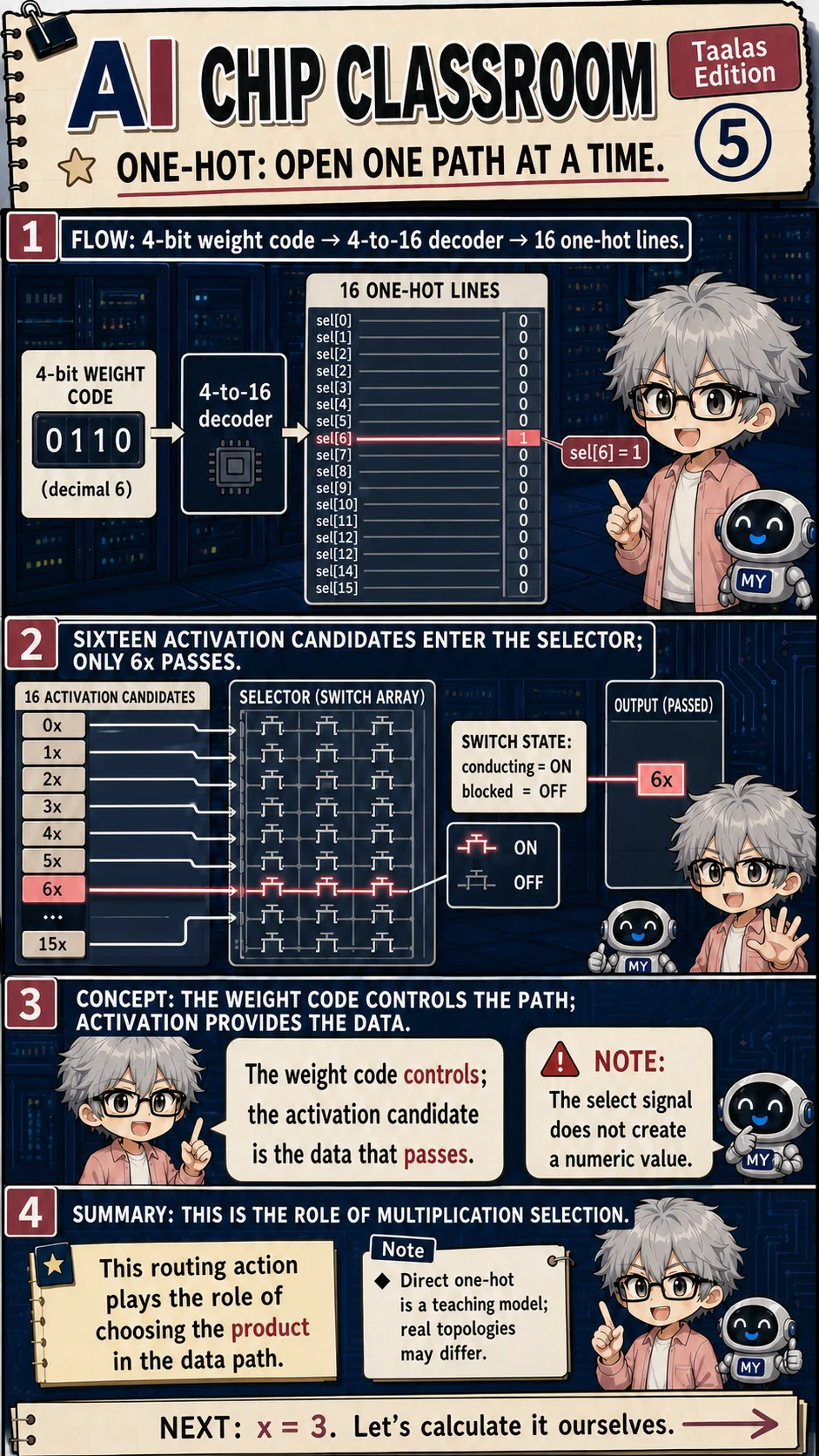
Take weight code 0110: decimal 6. After a 4-to-16 decoder, only sel[6] is 1 among the sixteen one-hot lines. The name is literal — one line hot at a time.
Sixteen activation candidates enter the selector array. The comic draws switches: on means pass, off means blocked. Only 6x is released. The switches do not carry product values; those values already sit on the candidate wires. Control comes from the weight; data comes from the activation side.
Direct one-hot is the clearest drawing. Real designs may use tree muxes or other encodings to ease routing and fan-out, so transistor counts on the page are not HC1 gate counts. Path count grows as 2^n: 8 paths for 3-bit, 16 for 4-bit, 256 for 8-bit — a cost plate 9 will reopen. The decoder itself still costs gates and wires.
The weight opens a door; the number still travels from the activation side. Do not confuse the switch with the multiply. Next, a worked table for x = 3.
Set x to 3 and look the products up

For x = 3, the entries 0x, 1x, 2x, 3x, 4x, 6x, 8x are 0, 3, 6, 9, 12, 18, and 24. The shifted ones are easy to spot: 2x=6, 4x=12, 8x=24. Build once, then look up repeatedly.
Pearl, milk tea, and coffee are three different weights on this plate — not three drink dimensions: w = 6 (0110), w = 8 (1000), w = 2 (0010). They point at 18, 24, and 6. The arithmetic is unchanged — 3×6=18, 3×8=24, 3×2=6 — but the products were prepared first, and each weight only selects.
The yellow caution on the plate matters: unsigned 4-bit teaching range 0–15, no negatives. Real matrix multiply still needs signed values, scaling, saturation, accumulator width, and per-layer ranges. The toy proves lookup can reproduce products; it does not prove an LLM runs on one sixteen-slot table.
The next plate flips the same mnemonic: pearl, milk tea, and coffee become output candidates, while inputs become milk-tea / sweet / chewy dimensions. Roles swap; the arithmetic does not. Build the table once; after that, every weight only chooses.
Look up every dimension, then add
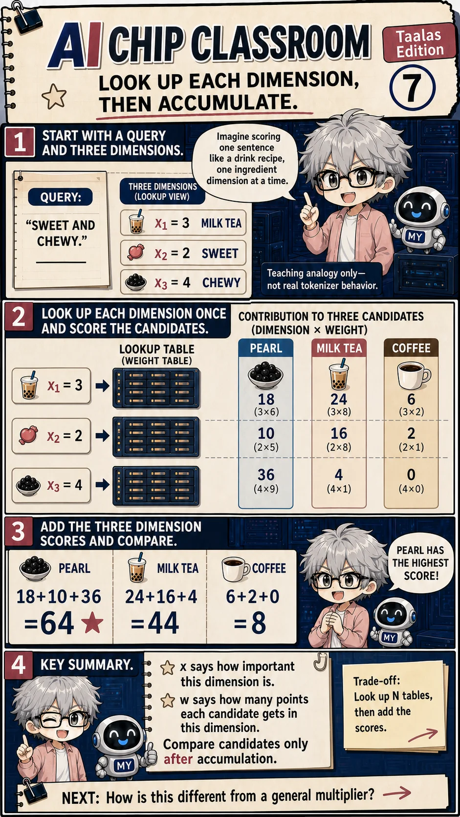
A matrix-vector product does not finish after one lookup. Treating a sentence as a milk-tea order gives three input dimensions as ingredients: x1 = 3 (milk tea), x2 = 2 (sweet), x3 = 4 (chewy). The plate labels this as metaphor, not tokenizer behavior — language models do not expose three hand-labelled dimensions with those names.
Each x gets a table, then pearl, milk tea, and coffee each take a score. Check the arithmetic: pearl is 3×6=18, 2×5=10, 4×9=36. Milk tea is 3×8=24, 2×8=16, 4×1=4. Coffee is 3×2=6, 2×1=2, 4×0=0.
Sums: pearl 18+10+36=64, milk tea 24+16+4=44, coffee 6+2+0=8. Pearl wins. The drink shop is a hook. The engineering point is that output channels wait until every input dimension has contributed.
x says how important this dimension is; w says how many points a candidate gets here; comparison comes last. The plate also writes the cost: N lookups, then a sum. Hardware usually does those dimensions in parallel; the comic serializes them so each term's origin stays visible. Share one x, select, accumulate, then move to the next x — that is the loop.
The mathematics stays; the reuse changes
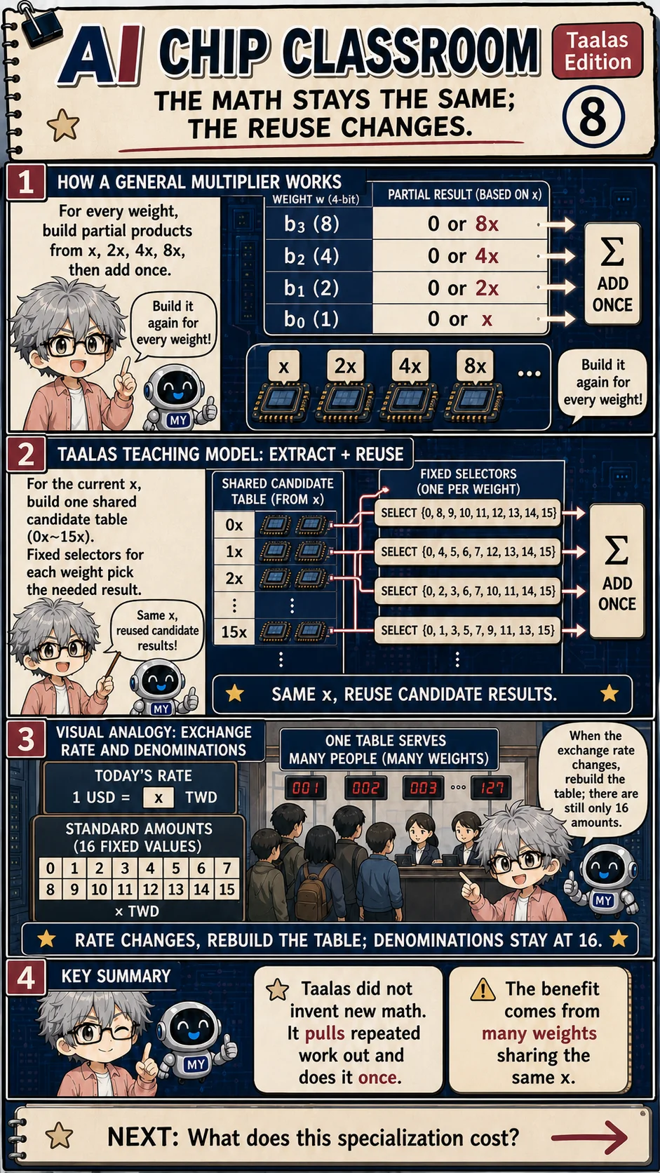
After the accumulation plate, the ordinary multiplier is easier to compare. Each bit of a 4-bit weight decides whether to add 8x, 4x, 2x, or x, then sums — already shifts and partial products. The waste, when weights are many, is doing the same x, 2x, 4x, 8x work over and over.
The shared-table side pulls that repeated work into the middle. Build one 0x–15x table for the current x, then feed a row of fixed selectors. Candidates are reused. Accumulation still happens. Partial products are no longer rebuilt per weight.
The FX counter is only a mnemonic. Today's rate, 1 USD = x TWD, is the current activation; the sixteen denominations are the low-bit weights; the queue is many fixed weights sharing one table. Change the rate, rebuild the table; the set of denominations is still sixteen. Do not read this as foreign-exchange hardware.
This classroom is not a new algebra. It extracts repeated work and does it once. The gain needs many weights sharing the same x. Narrow activations, awkward codebooks, weak sharing, or routing that dominates timing can shrink the advantage. A 2026 study of lookup-table accelerators for 1.58-bit LLM inference found that the best architecture depends strongly on activation data type; reuse helps less for small integer activations. That paper is related design-space evidence, not an HC1 schematic. [4]
The result is still x times w. What changed is which intermediate values are worth generating once, and which are still cheaper to redo per weight. Next plate opens the bill for specialization.
Specialization is fast, and it has a bill

Path counts from plate 5 unroll here. Direct one-hot: 3-bit gives 8 paths, 4-bit 16, 8-bit 256. Growth is exponential in bit-width. Real topologies may differ — this is a stress test of the teaching model, not a proof that 8-bit one-hot is always more expensive than a multiplier. That comparison needs area, congestion, and energy numbers this cartoon does not provide.
Three locks sit side by side. Low-bit quantization keeps the path count in range. Sharing one x amortizes table generation across many weights. Fixed weights let the data path specialize deeply. Drop one lock, and this story gets much less convincing.
On the scale: less data movement and reused candidates on one side; redesign and another tape-out, higher NRE, and less flexibility on the other. Shifts still have wires and load; precision and flexibility trade; only a stable model is worth this much specialization. Those are not late disclaimers — they are the other face of the same choice.
The last plate practices reading HC1's public numbers instead of memorizing them.
Engineer extension: PPA and updateability are the real closure targets
Architecture reviews must count more than multipliers. Candidate generation, decoders, selector networks, fan-out, buffers, accumulators, clock trees, placement, routing congestion, timing closure, and testability all enter PPA.
Fixing weights in masks or physical logic also turns model versions, bug fixes, security updates, and supply lifetime into product constraints. Hardwired inference fits best when demand is stable, volume can amortize NRE, and the model replacement cycle is predictable.
HC1: specialization pushed far, numbers read with their boundary

Public HC1 demonstrator specs on one card: Llama 3.1 8B, TSMC 6nm, 815 mm², 53 billion transistors; a 2.5 kW server; about 17K tokens/s/user. Read the warning printed on the plate with the number: stated test conditions, not an independent benchmark. [2]
The product page calls HC1 a technology demonstrator. The 17K figure is under 1K input / 1K output. Competitor numbers are not always measured the same way, so "how many times faster" should not harden into a universal constant. Card power, a ten-card server, batching, per-user latency, and throughput also have to stay un-mixed. [2]
The five-step recap ties the earlier plates: weights fixed in silicon; 4-bit codes, sixteen candidates; build the table; weight selects a route; accumulate across dimensions. Multiplication did not become magic. Model specialization is used to drop repeated movement and repeated arithmetic. The plate's own analogy is select-in-memory, compute-in-periphery, labelled as this article's phrasing rather than a standard industry name.
Whether this stance scales depends on tape-out speed, yield, cost, how often the model changes, and independent measurement under real serving loads. Vendor numbers are a starting point. They are not the verdict.
Five closing sentences
- Taalas fixes one model's weights and dataflow into silicon. The trade is efficiency against flexibility: less weight movement, and a model change often means redesign or another tape-out.
- A 4-bit weight has 16 codes, so candidate products for one activation can be reused. The plate's “150,000 requests” is classroom scale for “a lot,” not a product spec.
- One-hot and the 16-entry table are the teaching model. They separate control from data. They are not a public HC1 schematic.
- Shifts avoid a general multiplier and still cost wiring, load, area, timing, and accumulation. “Free” is a nickname that misleads.
- 17K tokens/s/user, 815 mm², 53B transistors, and 2.5 kW are Taalas's published figures. Read them with the model, sequence length, power, and test source attached.
Two optional next questions: how much room remains for LoRA, KV cache, and version updates after a model is fixed; and how lookup, selectors, routing, and accumulators close PPA. Pick one. Keep the habit: plates for intuition, numbers with their boundary, specialization is not a free lunch.
References
- Taalas, The path to ubiquitous AI: Official description of total specialization and HC1's system positioning.
- Taalas, HC1 Technology Demonstrator: Official model, process, die, transistor-count, server-power, performance, and test-condition figures.
- EE Times, Taalas Specializes to Extremes for Extraordinary Token Speed: Public discussion of 4-bit parameters, multiplication-related work, and fully digital operation.
- Geens et al., Hardware Generation and Exploration of Lookup Table-Based Accelerators for 1.58-bit LLM Inference: Related research on LUT accelerator design space and activation-data-type trade-offs; not an HC1 implementation description.
Exercise: sixteen candidates and fixed selectors
Three activations each build a 0x–15x candidate table. Two outputs select and sum products using fixed weights. Change the requested first weight, check whether the old selectors still match, then recompile the selectors.
A functional model with unsigned four-bit codes and exact integer arithmetic, not HC1 transistors, RTL timing or a quantized LLM. Overflow, scaling, wiring cost and fan-out are omitted. “Recompile” changes only this page’s array. Real fixed-model changes may require redesign and fabrication; configurable product features are a separate case.
Learning guide
AI Technology Classroom
Prerequisites
- Basic matrix-vector multiplication and low-bit quantization
What I learned
- Explain why fixed low-bit weights enable candidate-product reuse
- Walk a 4-bit weight from table build through one-hot selection and cross-dimension accumulation
- Read HC1's public numbers with their test boundary, without treating the plates as a chip schematic