One machine converts faster; another handles more photos at once
A photo studio is choosing a new server. Two candidates have very different core counts but similar public composite scores. Customers sometimes submit a single urgent photo and sometimes upload a batch. Should the studio prefer faster individual conversions or more cores? Consider whether a similar total score answers both needs.
This is a teaching scenario, not a product measurement. Following the single-core lesson on IPC and waiting, we now ask how multiple cores share the work. We follow that question through shared data, AI workflows and cost, then return to the purchase decision.
Reading guide: the comics introduce each question; the article develops its conditions, examples and decisions. Talk observations are attributed, and teaching numbers are not product measurements.
Why are CPUs back in the discussion?

If GPUs run model computation, why discuss CPU performance in an AI system? Data preparation, tool calls or scheduling can delay later stages. More GPUs alone may not improve the completion rate. Debbie starts her talk from this changing demand and argues that CPU performance deserves renewed attention. The design question is whether expensive compute resources can receive their next job.
The opening summarizes observations relayed at ISCA 2026. CPU/GPU ratios are not universal configurations. Debbie also relays a core-demand forecast: requirements previously discussed as fourfold were later described as eight- to tenfold. That is not another eight- to tenfold increase on top of the fourfold level, nor growth measured in this lesson. We first build a way to judge latency and completion rate using the photo studio, then return to AI, ISA choices and demand.[9]
What are we measuring: one job or a whole batch?
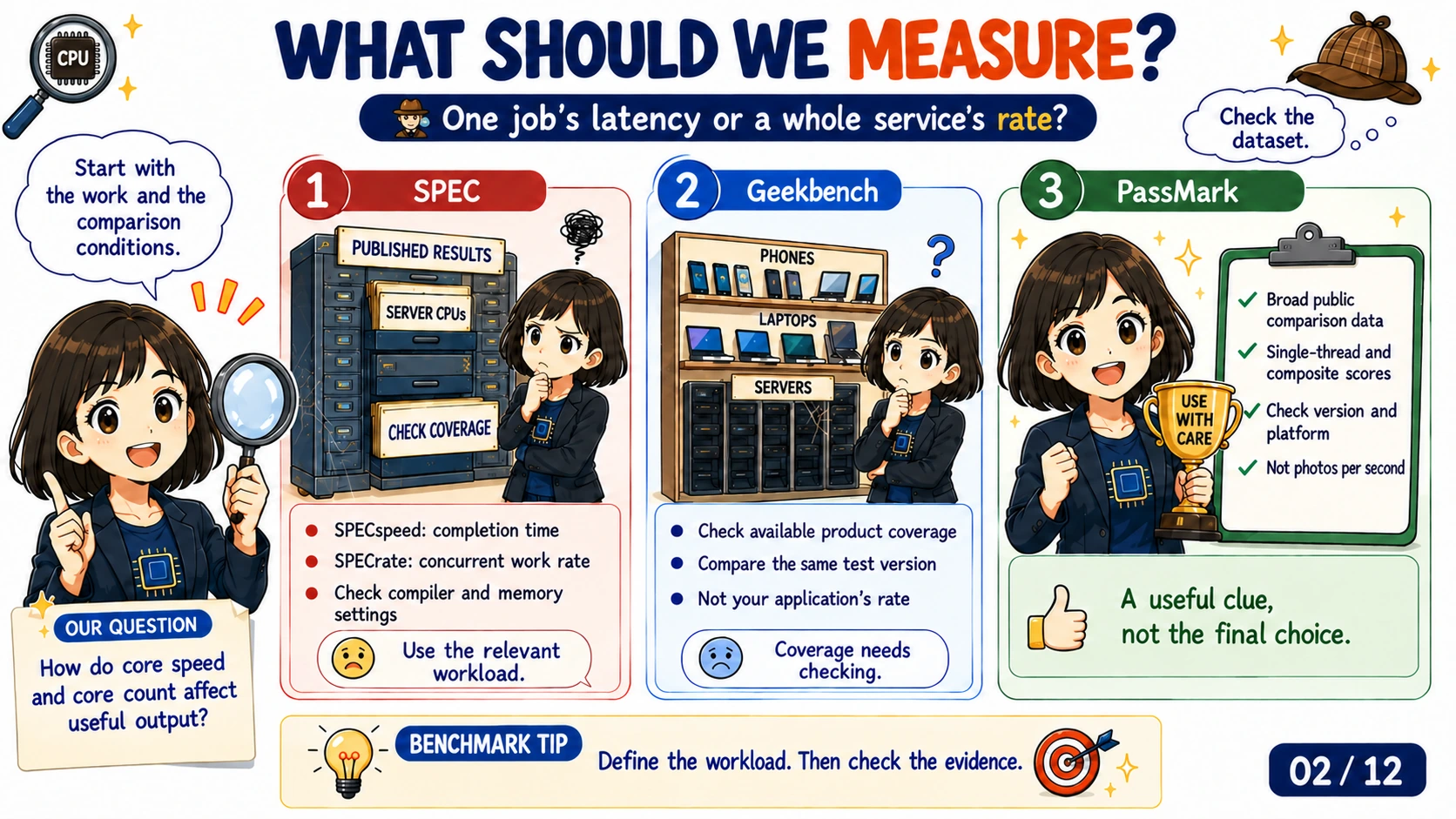
Photo conversion gives us two different performance questions. Someone submits one image and wants the result quickly. The time they wait is latency. A studio with a large queue asks how many images it can finish each second. That completion rate is throughput. Adding cores can let the studio process more images at once without making the computation for any one image faster. We need to measure both questions separately.
Standard benchmarks make a related distinction. SPEC CPU2017 uses SPECspeed to focus on completion time and SPECrate to assess how quickly multiple copies of a workload finish. It sets execution and reporting rules, but results still depend on compilers and the memory system. A product label such as phone or server does not, by itself, establish whether a benchmark is useful for a question.[1]
The retained scatterplot uses PassMark scores. A single-thread score gives evidence about performance under its particular tests. CPU Mark combines several tests. A score of 60,000 does not mean 60,000 converted photos per second and cannot be substituted for service throughput. Before comparing results across software versions, operating systems or compilation conditions, check how the scores were produced.[2]
The studio can use public scores to shortlist machines, then run the same photo batch on each candidate. Keep image size and output quality fixed. Measure completion rate and individual waiting time, and verify the output. If public data does not cover a candidate product, missing results do not establish poorer performance. The test and its actual data must fit the question.
How do more cores increase the completion rate?
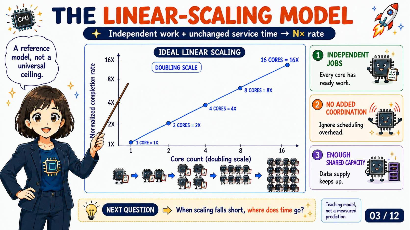
Suppose one core takes one second to convert a photo. Photos are independent and the queue always has work ready. Its ideal completion rate is one photo per second. Four identical cores can each process a different photo, giving four photos per second in the ideal case. The computation for each photo still takes one second. Higher throughput has not reduced its individual computation time to a quarter of a second.
This teaching example temporarily excludes scheduling and data-delivery costs. A real program must expose work that can run concurrently and let the operating system schedule it. Four cores cannot automatically divide a dependent instruction sequence into four independent parts. Hardware threads also differ from physical cores. With SMT, threads share some core resources, so more threads do not guarantee a matching multiple of performance.
Under those ideal conditions, one core finishes 100 photos in 100 seconds; four cores finish them in 25 seconds. That is speedup for the batch. If the program has only one photo and assigns the entire conversion to one core, it gains no such speedup. Extra capacity can nevertheless reduce queueing delay in a busy service. A user's total wait may fall even though the photo's computation time has not changed.
The linear curve is a reference for testing these assumptions. If four cores deliver only three photos per second, first check whether enough work is ready, then identify the constraint. Busy cores may spend time synchronizing or waiting for data instead of doing useful computation. Conversely, a working set that fits in more aggregate cache can sometimes produce apparently superlinear scaling. The curve is a simplified reference, not an absolute ceiling for every system.
Why does the same roughly 60K score not establish core equivalence?

At 42:18–42:50 in her talk, Debbie Marr compares 18 high-performance cores, Grace's 72 cores and Ampere's 192 cores within a band near 60K. The artwork uses that observation to show that core count and total score have no one-to-one relationship. These numbers have a source, but the transcript does not supply the full point ledger, every product identity or test settings. June 26, 2026 is the inherited chart's snapshot label, not a new measurement. We do not treat the comparison as independently verified product equivalence or infer a tenfold per-core advantage for an architecture.[9]
Use a teaching example we can calculate instead. Machine A has four cores, each converting two photos per second. Machine B has eight cores, each converting one. With independent work and sufficient data delivery, both ideally finish eight photos per second. A's computation time per photo is half a second; B's is one second. Equal aggregate completion rates can coexist with different individual latencies. That difference matters when a customer has a delivery deadline.
Per-core performance can change when many cores run together. All-core frequency may be lower than single-core boost frequency, and cores may share caches and memory. Multiplying a single-thread benchmark score by core count misses these conditions. A processor with different core types adds another complication: estimate the work rate of each type rather than treating every core as an identical unit.
An initial throughput model sums the effective completion rates of the workers, then checks whether shared resources reduce those rates. This is a starting point for analysis, not a replacement for measurement. The photo studio should compare completed images per second, delivery time and cost at equal output quality. Similar scores in the retained chart suggest questions to investigate; they do not decide which machine suits this workload.
Where does the time go after adding cores?
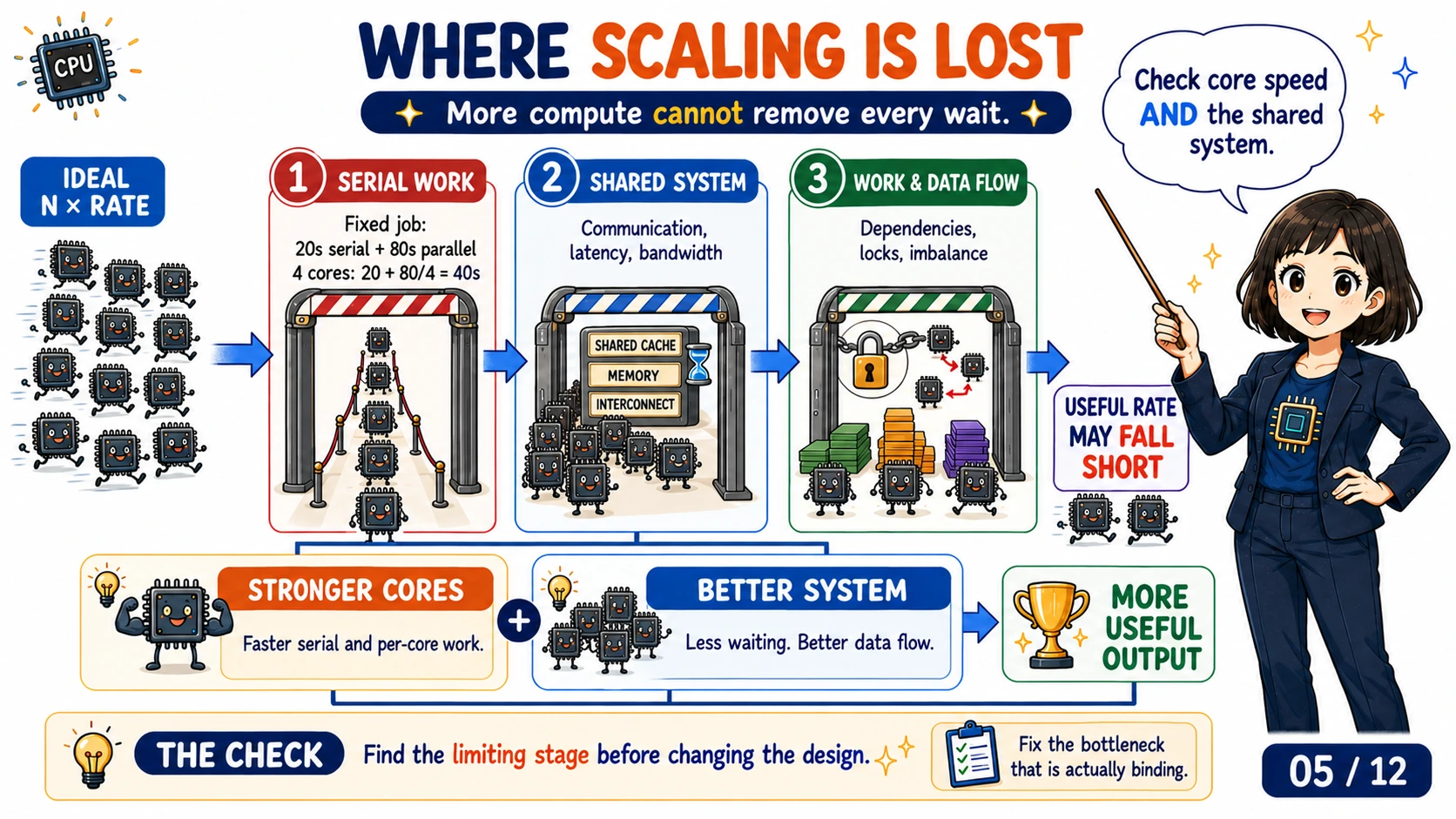
A batch that must finish as one job can be limited by serial steps. Suppose the single-core run takes 100 seconds. A common initialization takes 20 seconds and must run sequentially; the remaining 80 seconds divide perfectly across four cores. Ignoring extra overhead, completion takes 20 + 80/4 = 40 seconds. Speedup is 100/40 = 2.5. Even if the parallel work became almost instantaneous, the 20-second portion would leave a fivefold speedup limit. This is a fixed-workload Amdahl model.[3]
That common initialization differs from sequential steps inside each independent photo conversion. Different photos can still run on different cores. The Amdahl example concerns the completion time of one fixed job. A continuing service needs a separate check for shared bottlenecks. If every photo passes through one serialized output stage that can write only two photos per second, more conversion cores cannot sustain eight completed photos per second at the output.
Shared data paths can constrain scaling too. Cores moving large amounts of image data may saturate memory channels before exhausting their compute capacity. Additional cores then increase waiting. If cores repeatedly modify shared state, cache coherence must keep their copies consistent, potentially moving ownership and data between cores. Those delays differ from the time spent executing instructions inside a core. Higher IPC alone cannot remove them.
Uneven work leaves some cores idle. Assign four differently sized photos permanently to four cores, and the core processing the largest may be the only one still working near the end. Smaller work units or a shared queue can help workers take new jobs as they finish. Splitting and synchronization also cost time. Diagnose the bottleneck before choosing a core upgrade, data-layout change or scheduling fix. CPU utilization alone usually cannot distinguish these causes.
Engineer extension: efficiency, NUMA and false sharing
For a fixed job, speedup is S(N) = T(1)/T(N), and parallel efficiency is E(N) = S(N)/N. The four-core example gives 2.5/4 = 62.5%. This efficiency is not performance per watt. In a NUMA system, memory-access cost depends on the node holding the data, so thread placement and data allocation need to be considered together. Separate variables placed in one cache line can also trigger false sharing through repeated writes. The next Cache & Coherency lesson develops these mechanisms; an aggregate score cannot diagnose them.
How does performance become product value?
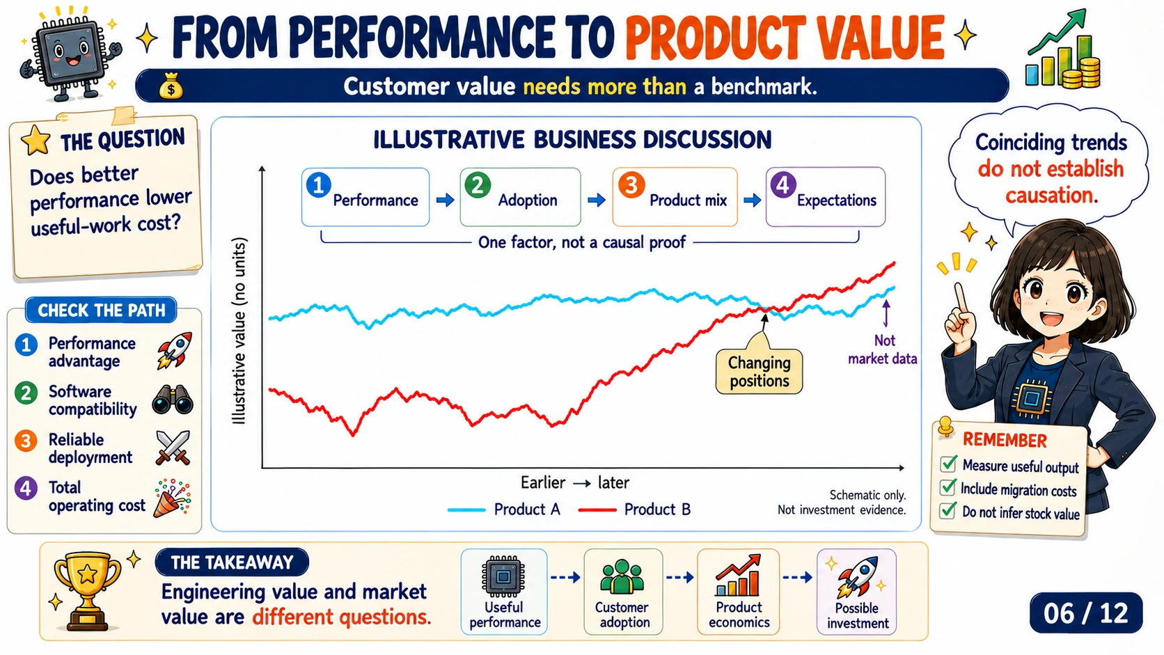
The studio ultimately needs to deliver the required photos within its budget. That is where performance can become business value. If it could meet the same quality and deadline with half as many machines, it might save equipment or rack costs. It must weigh those savings against purchase price, power and maintenance. A higher benchmark score alone does not establish a lower operating cost.
A processor supplier also needs to turn performance into a product customers will adopt. Customers check whether their software runs and whether systems are supplied reliably. An advantage accompanied by expensive software migration may see limited adoption. Compatibility and long-term support can also make a product with a lower peak score attractive. These are conditions for product decisions, not financial forecasts about any company.
Debbie's original talk discusses Intel and AMD when linking performance leadership to business outcomes. This page uses unitless Product A/B curves to retain the question of changing competitive positions without presenting a verified market-cap record. Even two accurate concurrent trends would not automatically establish causation. Product mix and manufacturing strategy can affect company outcomes too. Market capitalization reflects future expectations and differs from current cash flow.[9]
The useful question here is why a customer would pay for a particular performance advantage. The studio can partly answer it by measuring cost per acceptable photo, then checking delivery reliability. Whether a supplier consequently earns more revenue or gains research resources requires separate business evidence. The artwork starts a discussion; it is not investment advice and cannot support a claim that a faster CPU necessarily produces a higher market value.
When does a CPU actually keep a GPU waiting in an AI workflow?
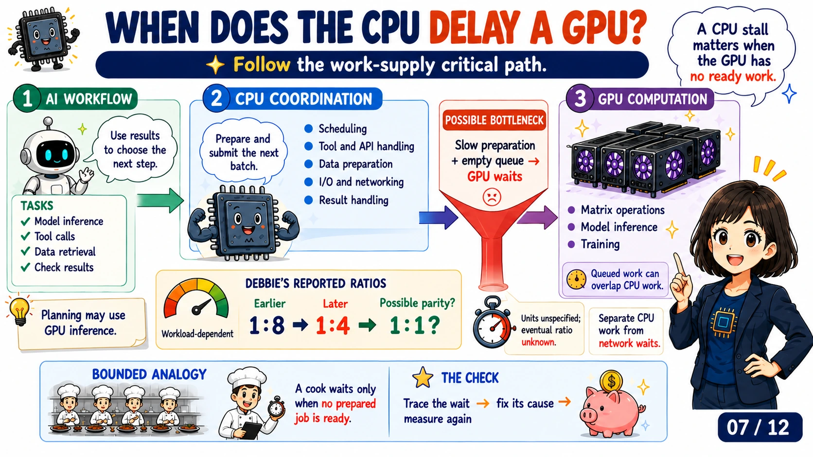
Now consider a photo service with several AI steps. A model identifies image content, software calls a tool to modify the image, and a model checks the result. Such workflows, which choose later actions from earlier results, are often called agentic AI. Recognition or planning may run as model inference on a GPU. A host CPU may receive requests and assemble tool results. The split depends on deployment; understanding and planning cannot all be assigned to the CPU.
Suppose the CPU must prepare the next GPU batch and the GPU's existing work queue has emptied. Slow preparation then makes the GPU wait. This is the same work-supply bottleneck we saw in photo conversion. If the CPU is waiting for a remote tool response, however, the delay may originate in the network or external service. A faster core might not reduce it. Trace the wait to its actual source first.
This condition also shows where the kitchen analogy stops applying. A GPU can execute work already submitted while the CPU prepares the next batch. Independent requests may fill one another's gaps. NVIDIA's asynchronous-execution documentation explains such overlapping work, subject to dependencies and hardware capabilities. A one-millisecond CPU pause does not necessarily idle every GPU for one millisecond.[4]
At 25:15–25:43, Debbie relays the Intel CEO's comments about CPU/GPU ratios: from 1:8 to 1:4, potentially approaching parity. She then says she does not know the eventual ratio. This is a sourced industry observation and forecast, not a configuration law for all AI systems. The passage does not define whether CPUs mean processor packages, core counts or another unit. First measure whether the GPU lacks work, waits for data or is fully loaded, then size CPU capacity. Do not choose equipment from those three ratios alone.[9]
How should we evaluate a RISC-V opportunity?

If the studio considers a RISC-V server, its first question is whether the same photo software can run there. An instruction set architecture, or ISA, defines instructions and software-visible behavior. Branch prediction, instruction scheduling and cache design belong to the implementation. One ISA can support small cores and more complex ones. Its name alone cannot predict single-core latency or multi-core completion rate.
The open RISC-V ISA gives designers implementation choices. Use of the ISA does not make an entire chip or commercial core IP free; other IP and software support may still carry costs. GCC provides RISC-V target options for extensions and ABI choices. That establishes toolchain support, but it does not establish that every package or optimized library can be moved unchanged.[5] [6]
Multi-threaded software also needs correct synchronization. At 54:39–54:57, Debbie contrasts strong and weak ordering, then describes Arm and RISC-V as having a common memory model. In context, this lesson interprets that as a shared weak-ordering concern and potentially useful porting experience. That is a teaching interpretation, not knowledge of her position on every rule. At the specification level, RISC-V's base model, RVWMO, cannot be equated with Arm's rules. RISC-V's official porting guidance separately maps Arm acquire and release operations. Atomics and synchronization still need target-specific validation.[7] [9] [11]
The knight battle presents ISA competition as a historical story, but the next P6 remains an analogy. The 30,000+ applications do have a source: at 48:37–48:59, Debbie cites Google's migration work, and Google's own report confirms more than 30,000 applications migrated from x86 to Arm. This demonstrates progress on a large-scale ISA migration, not an equivalent result already achieved on RISC-V. The studio must still check target packages and test correctness and performance. AI can help change code but cannot replace validation. An opportunity for a new ISA must be established through those steps.[9] [10]
Does cheaper software necessarily increase compute demand?
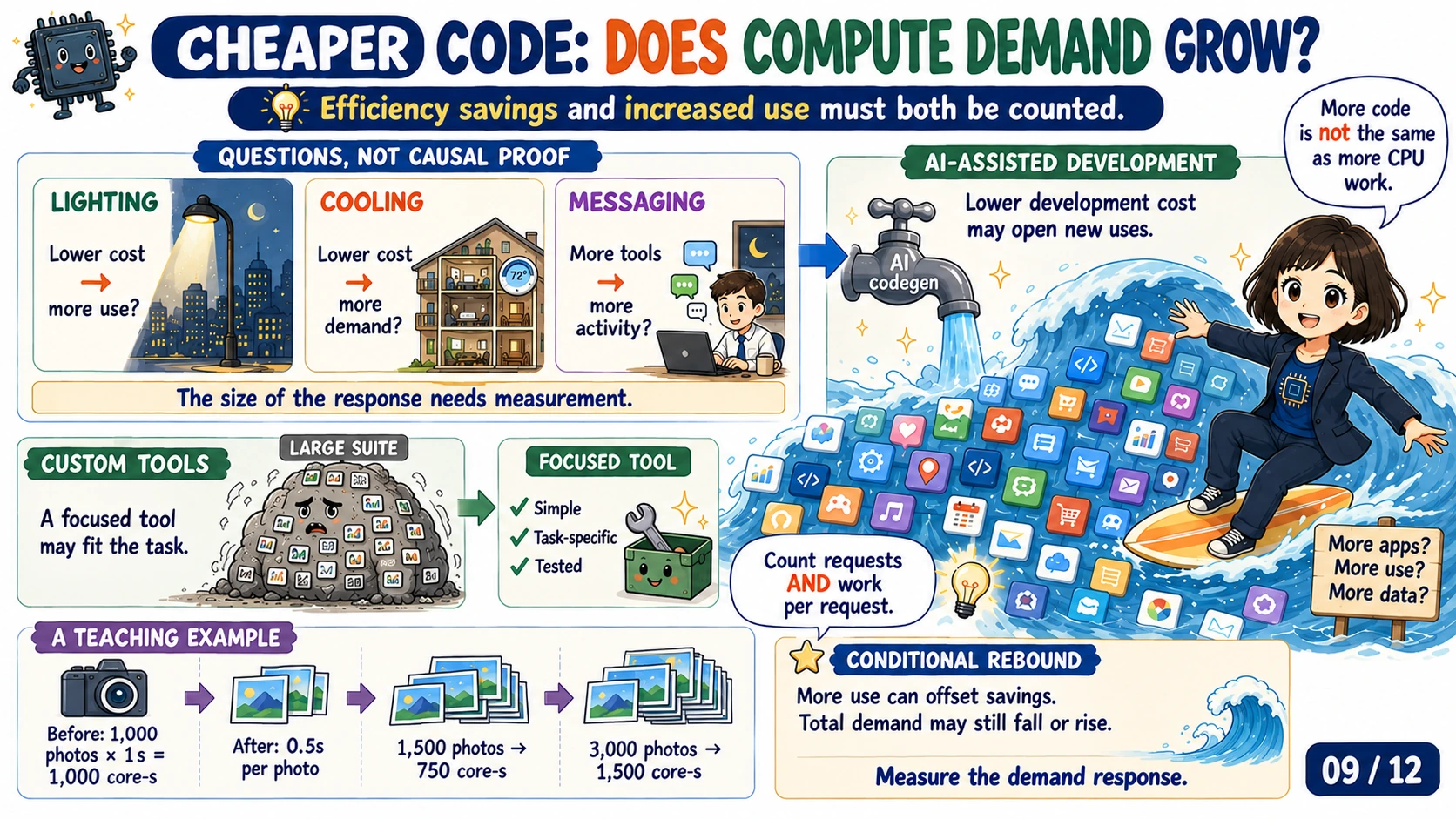
The studio may previously have found custom tools too expensive to develop except for a few workflows. If development becomes cheaper, it may build more tools, perhaps to organize filenames or check delivery formats. That is one reason demand could expand. How often those programs run and how much computation they use are separate questions. More generated code does not immediately imply a proportional increase in CPU demand.
When increased use offsets some resource savings from improved efficiency, we call it a rebound effect. If the additional use exceeds the savings, total resource consumption rises: the outcome commonly associated with Jevons paradox. Rebound can be partial without reversing the savings. The concept therefore does not guarantee that greater efficiency increases total consumption. Economic research treats the demand response as something to analyze.[8]
Calculate it for the same photo workload. At one second per photo and 1,000 photos a day, demand is 1,000 core-seconds. After an improvement, each photo takes half a second. If demand grows to 1,500 photos, total computation is 750 core-seconds, still below the original amount. At 3,000 photos it becomes 1,500 core-seconds. These teaching numbers show that the same per-item efficiency gain can produce different aggregate outcomes.
AI lowering the cost of some development tasks may open previously uneconomic uses. It may also create rarely used tools or make existing programs more efficient. The artwork's lighting, air-conditioning and messaging examples suggest questions; they do not establish that efficiency caused those lifestyle changes. For server capacity planning, measure actual request volume and work per request, then estimate how each may change.
How do we choose core strength, core count and cost together?
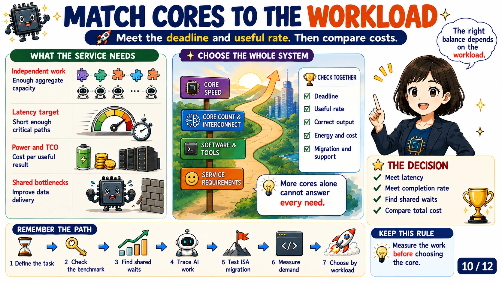
Return to the two machines that each finish eight photos per second. A takes half a second to compute one photo; B takes one second. If the customer requires delivery within 0.75 seconds of submission, B misses the requirement even before queueing is considered. For an overnight batch that only needs to finish before morning, B could remain a suitable candidate. Service requirements determine the value of a core design.
Costs can differ too. Suppose A draws 200W at the system level and B draws 120W under the same sustained workload. Both complete eight photos per second, giving approximately 25J per photo for A and 15J for B. This is a teaching calculation at fixed quality and equal throughput, not a product measurement. B's better energy result does not remove its earlier latency limitation.
Total cost of ownership, or TCO, combines purchase and continuing use. Power is one part; maintenance, software and deployment contribute too. Divide total cost by the acceptable work completed over the period to compare cost per delivery. Include software migration or additional machines needed to meet deadlines. A peak benchmark score or a single performance-per-watt score cannot replace that system-level calculation.
Choose core strength and core count together. A serial critical path benefits from lower latency; many independent jobs need enough aggregate capacity. Improving cores may have little effect when shared data delivery is the constraint. Looking only at core speed or only at core count omits those conditions. Our design rule is to meet service requirements first, then compare useful throughput and cost. It does not prescribe a few large cores for every workload.
Back at the studio: which bottleneck should we fix first?
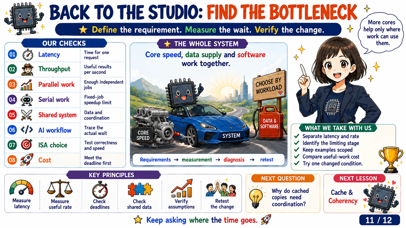
The studio can now state its purchase problem precisely. Define photo quality and the individual delivery deadline, then the daily work volume. Measure computation time, queueing delay and completion rate separately. If equal frequencies produce different conversion times, the previous single-core lesson's discussion of IPC and data waiting gives us a direction. If adding cores fails to improve completion rate, this lesson's parallel-work and shared-bottleneck checks provide the next steps.
When each core has independent photos and memory supplies the data, more cores can increase capacity. If every photo waits for one output stage, improve that stage first. If only one core remains busy with the final large image, inspect work partitioning. If the delay occurs at a remote service, measure network and external-response time. Similar low-throughput symptoms can have different causes, so fixes must follow the cause.
Change one condition to test the explanation. Photos were independent, but now they must contribute to a shared statistical result. Each core can calculate a partial result, followed by a merge. A long sequential merge can constrain batch completion time. The earlier linear-scaling assumption no longer holds. Measure this new stage before deciding whether additional cores still help.
This lesson does not develop coherence-protocol state transitions, derive queueing theory or evaluate particular products. Continue with the Cache & Coherency classroom: why must cores communicate when they hold copies of the same data? Connecting that question to this lesson explains why some waiting cannot be removed by adding cores alone.
Multi-core key points
- Latency measures the wait for one job; throughput measures completed work per unit time.
- Independent work can run concurrently; serial common stages and shared resources still constrain scaling.
- Composite scores provide clues, not product equivalence or deliveries per second.
- Find the actual work-supply critical path in an AI system; a CPU pause need not stop every GPU.
- Check quality, deadlines and cost before choosing a core design.
Hashtags
#CPU #MultiCore #Throughput #Latency #Amdahl #Scalability #AgenticAI #RISCV #TCO
References
- SPEC CPU2017 Overview — SPECspeed, SPECrate, workload and comparison conditions.
- PassMark PerformanceTest — CPU Benchmark — Test and aggregation methodology; does not reconstruct the inherited chart.
- Hill & Marty (2008), Amdahl’s Law in the Multicore Era — Fixed-workload serial fractions and multicore design analysis.
- NVIDIA CUDA Programming Guide — Asynchronous Execution — Conditions for overlapping host and device execution.
- RISC-V International FAQ — Open ISA versus implementation IP costs.
- GCC — RISC-V Options — Target settings for ISA extensions and ABI.
- RISC-V — RVWMO Memory Consistency Model — RISC-V ordering rules, not a synonym for the Arm memory model.
- Chan & Gillingham (2015), The Microeconomic Theory of the Rebound Effect and Its Welfare Implications — Demand analysis for energy rebound; its software application here is a conditional analogy.
- Debbie Marr, Computing at the Crossroads: Architecture, Economics, and the Next Era, ISCA 2026 official program. Content checked against the supplied talk transcripts: first file 25:15–25:43 (ratios), 26:10–26:28 (fourfold to eight- to tenfold core-demand forecast), 42:18–42:50 (core comparison), 48:37–48:59 (migration), 54:39–54:57 (memory model). Times start at that file’s beginning. The program identifies the session; it is not a transcript. Recognition errors remain, so ambiguous passages are not presented as verified audio.
- Google — Using AI and automation to migrate between instruction sets — More than 30,000 applications migrated to Arm while retaining x86/Arm support, not a RISC-V migration count.
- RISC-V — Code Porting and Mapping Guidelines — Official commentary mapping Arm operations to RVWMO. Commentary is not the normative specification, and the models should not be equated.
Meet the true CPU great master!
About the author — author/speaker of the original talk

Meet Debbie Marr. The ISCA biography records over thirty years of CPU development at Intel: Pentium Pro server architect, bringing Hyper-Threading to Pentium 4, and Haswell chief architect. She also directed Intel Labs' Accelerator Architecture Lab.[9]
It lists over thirty papers, forty patents and an electrical and computer engineering PhD. She co-founded AheadComputing in 2024 as CEO. That experience deserves attention; forecasts still need to be distinguished from measurements and specifications. MY Academy prepared and extended this lesson. This lesson is not presented as Debbie's endorsement.
Learning guide
CPU Classroom Series
Explore the complete 26-lesson CPU curriculum →
Prerequisites
- Single-core IPC and waiting
- Independent jobs can run concurrently
What I learned
- Distinguish latency, batch speedup and service throughput
- Calculate a fixed-workload Amdahl example and diagnose shared bottlenecks
- Separate composite scores from application throughput and product equivalence
- Choose core strength and count under latency and cost constraints