High-Performance Single-Core CPU Classroom: Why the Same GHz Can Be Twice as Fast

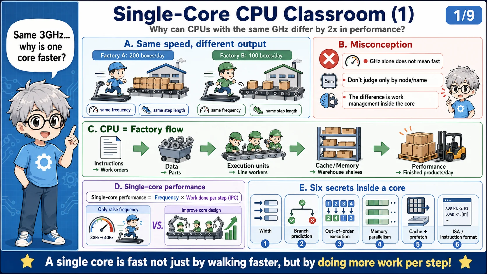
Same GHz does not mean same work per second

At 3GHz, a processor has about three billion clock cycles per second. A cycle is a unit of time in which hardware advances its work. It does not guarantee that the CPU completes exactly one instruction. Some instructions take several cycles. A core may also complete several instructions in one cycle. Cycle length alone cannot tell us when a program will finish.

Imagine two factories receiving the same batch of orders. Their workers move at the same pace, but factory A gets its materials on time. Factory B often stops to find supplies or wait for another order. A can finish more by the end of the day. In the CPU, instructions are work orders and data is material. Execution units perform operations. Cache holds frequently used data nearby. The frontend fetches instructions and decodes the requested operations.

We use IPC, short for Instructions Per Cycle, to measure the core's output. In this lesson, IPC is the number of retired instructions divided by the number of clock cycles. Retirement means the core formally accepts an instruction's result. Instructions discarded after a wrong prediction do not count toward that output. IPC is an average over an execution interval. It changes with the program being run.

The six mechanisms ahead address different waits. Width creates room for simultaneous work. Branch prediction prepares the next path. Out-of-order execution finds instructions that are ready. Memory-level parallelism keeps several requests in flight. Cache and prefetching supply data, while instruction format affects the frontend. These mechanisms interact. Their individual benefits cannot simply be added together.

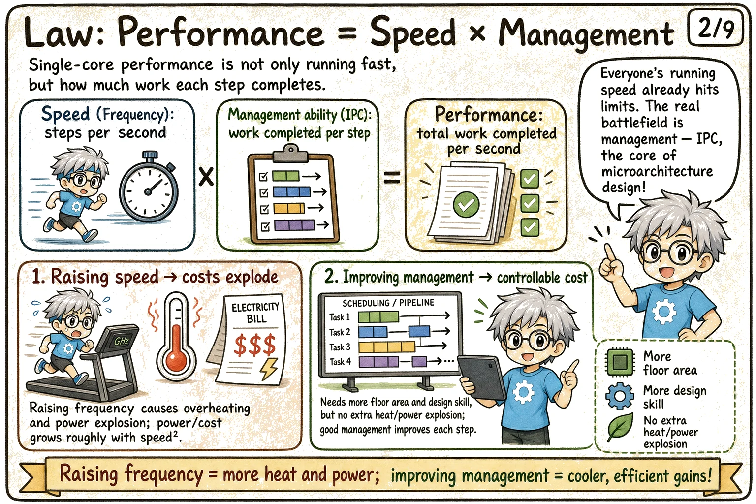
Frequency and IPC: calculating execution time

We can calculate how long the same job takes in three steps. Count the instructions executed and retired. Divide by average IPC to find the cycle count. Then use frequency to convert cycles into seconds. The relationship is execution time = instruction count / (IPC × frequency). The plate's speed-times-management analogy helps explain the denominator. Instruction count still matters when comparing different programs or instruction sets.

Try a simplified example. Both cores retire three billion instructions and maintain a 3GHz clock. Core A averages an IPC of 2; core B averages 1. A needs 1.5 billion cycles, or about 0.5 seconds. B needs three billion cycles, or about one second. These are teaching numbers and exclude other system waits. The twofold difference comes from cycle count, without increasing GHz.

A higher frequency can shorten each cycle. The circuits must then produce correct results in less time. Designers may need more voltage or a different pipeline partition. Dynamic switching power is often approximated as P ≈ αCV²f. Here, α is switching activity, C is effective capacitance, V is voltage, and f is frequency. This model excludes some leakage and system power. If voltage also rises, power can increase faster than frequency.

Higher IPC also has a hardware cost. More instruction-tracking space can expose more work. A wider frontend and additional execution units consume area and power. Designers must also verify that these resources cooperate correctly. A product balances performance against those costs. A fair comparison fixes the job and input, and records the compiler settings and execution environment. SPEC's reporting rules illustrate why these conditions matter. ^[2]

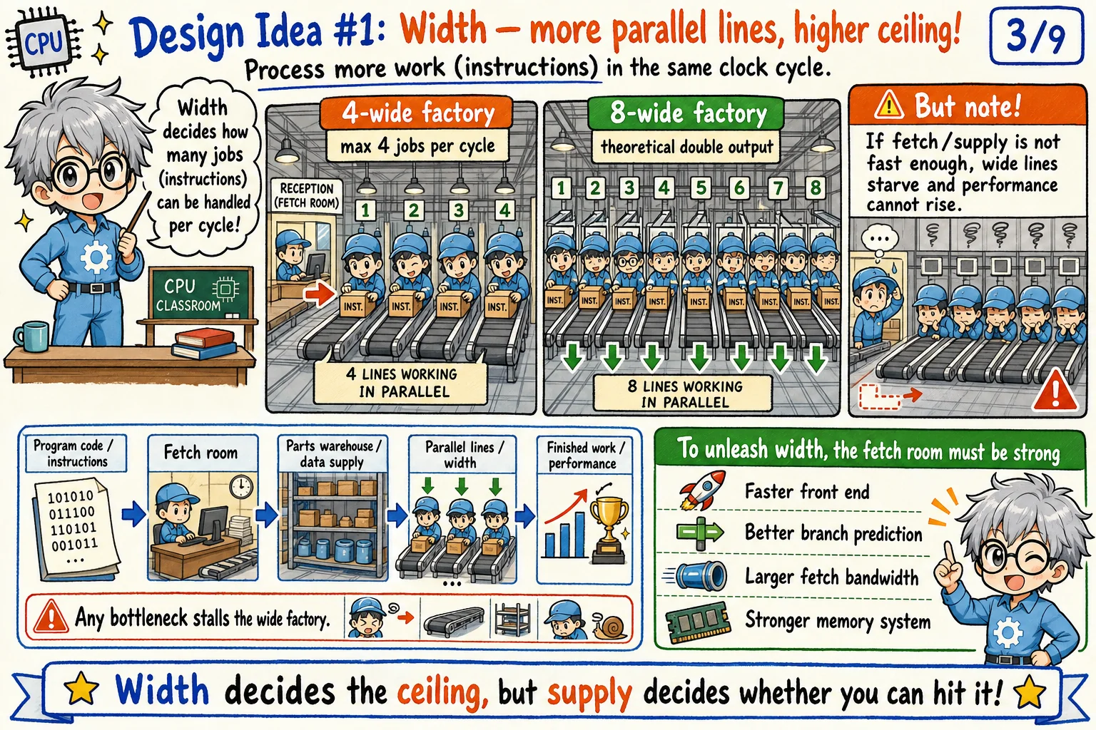
Width raises the ceiling, but supply decides whether you reach it

A factory can add production lines. A CPU can increase the number of operations it handles per cycle. This is called superscalar execution. However, a claim such as 8-wide must identify the stage being measured. Fetch, decode, issue, and retirement widths may differ. Some stages count micro-operations: internal units of work that do not necessarily match one software-visible instruction.

Treat the plate's 4-wide and 8-wide factories as simplified production lines. With eight prepared orders, eight lines may work together. If the receiving office supplies only two orders, the others sit idle. A CPU has similar supply problems. An instruction-cache miss makes the frontend wait. Slow decoding leaves the backend short of operations. Widening one stage may leave the throughput of the whole pipeline unchanged.

The program also limits parallel work. Suppose B uses the result of A, and C uses the result of B. These instructions form a dependency chain. Eight execution units cannot make B start before its input is available. Eight independent operations offer more opportunities. We call those opportunities instruction-level parallelism, or ILP. The core must find them and have suitable execution units available.

A wider design needs more data paths and control circuitry. Registers must support more accesses, and the scheduler must make more choices. These changes can increase power and make a high clock frequency harder to achieve. An 8-wide design therefore offers a higher limit at a particular stage. It does not promise twice the performance for every program. Our computer-selection example still depends on how much independent work the program supplies.

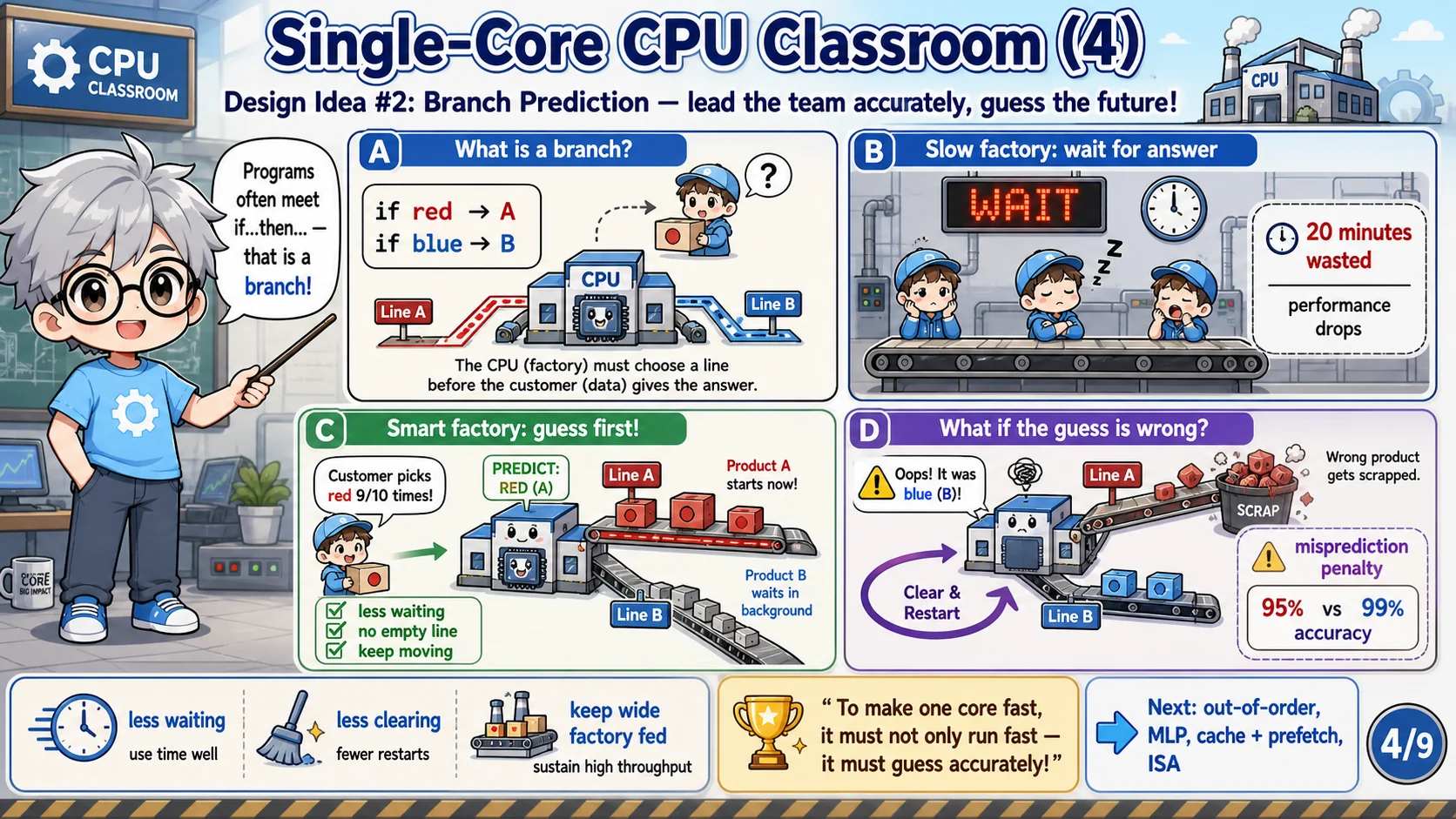
Branch prediction keeps the factory from waiting

A factory receives an order that says to process a part only if it meets a condition. The inspection must finish before anyone knows the answer. A CPU meets a similar problem at an if/else statement. Loops and function returns also change the next instruction address. If the frontend always waits for the answer before fetching instructions, execution units may run out of new work.

The branch predictor estimates the next instruction address. The core prepares work along that path and may execute it speculatively. Those results are not yet accepted as final. Once the condition resolves, the core checks its prediction. A correct prediction lets work continue. A wrong prediction requires discarding wrong-path instructions and restarting at the correct address. Preparing the correct work again takes time: the misprediction penalty.

The plate's 95% and 99% differ by four percentage points. Across one hundred predictions, the first accuracy means five errors; the second means one. That is an 80% reduction in error count. It does not make the whole program 80% faster. The speedup depends on how often branches occur and how much each error costs. Overlap with other waits also affects the result.

Prediction involves several questions. Direction prediction estimates which way a conditional branch goes. A branch target buffer, or BTB, helps find the destination. A return address stack, or RAS, helps predict function returns. A wider or deeper pipeline may waste more prepared work after an error. Designers balance accuracy against lookup speed and hardware cost. If our example program branches frequently, this is a useful place to investigate.

Out-of-order execution means ready work goes first

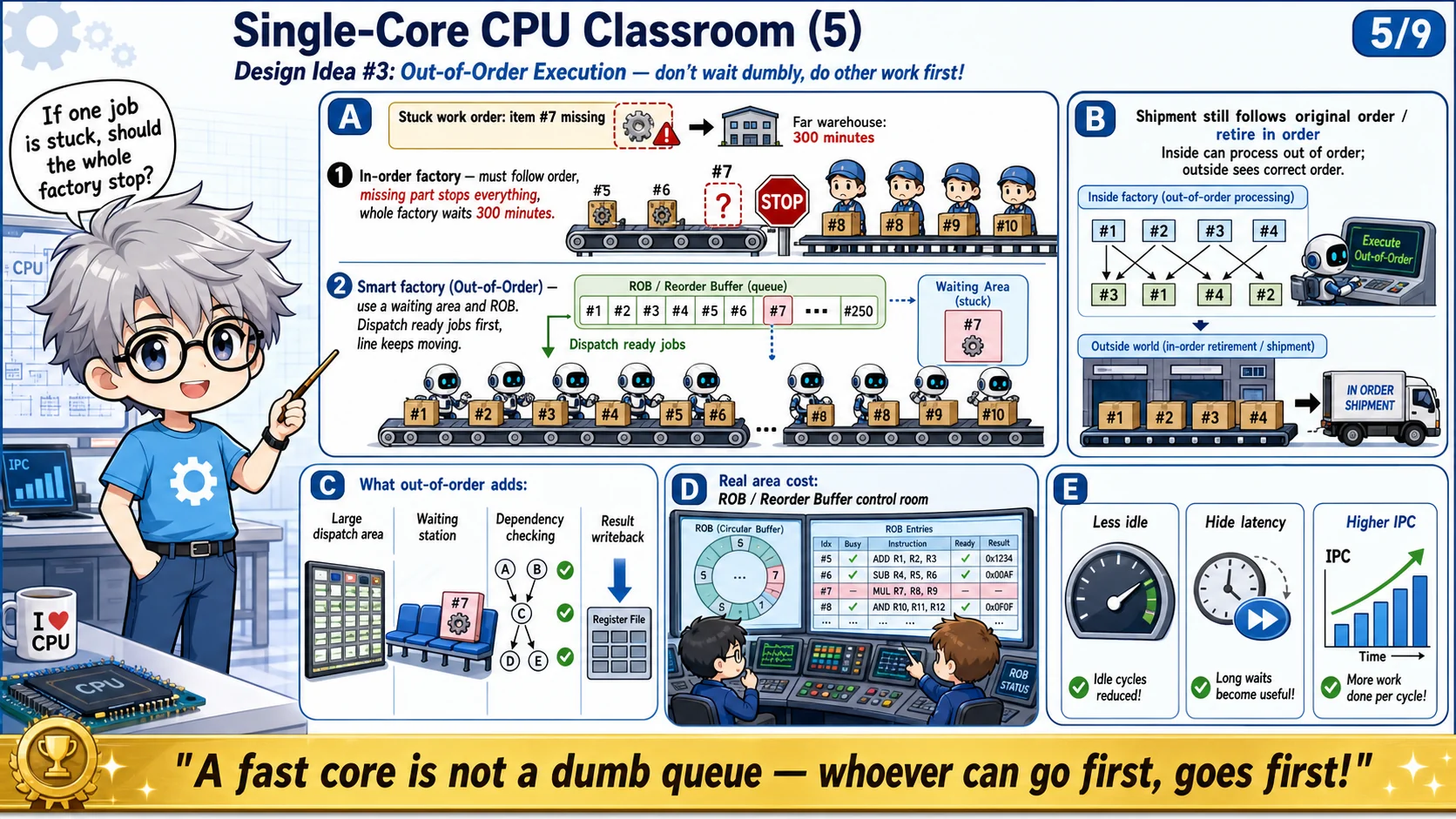
Consider another stoppage. Order A is waiting for material, but B, C, and D have everything they need. If the factory must start every order in sequence, those three orders wait too. An in-order core can encounter similar blocking. Its control is usually simpler. However, an early instruction that cannot advance may prevent later independent work from using idle execution units.

An out-of-order core examines a group of instructions that have not yet retired. The scheduler finds work whose inputs are ready and assigns it to available execution units. B, C, and D can then run while A waits. If B needs A's result, B must still wait. Hardware can exploit independent work, but it cannot remove a true data dependency.

Finishing an operation and retiring its instruction are separate events. The reorder buffer, or ROB, tracks the original instruction order. A typical out-of-order core retires instructions in order to accept their results. Register renaming separates reused register names. The load/store queue helps check memory dependencies. The core must also handle exceptions and wrong predictions correctly. The gem5 O3CPU model shows how these stages cooperate. In-order retirement does not require every memory operation to be issued in order. ^[3]

Tracking space is finite, so the core cannot search arbitrarily far ahead. If every instruction depends on A, the scheduler finds no alternative work. A long wait can also fill the ROB and stop further progress. A larger ROB and scheduler can look farther ahead. They consume more area and power, and require more verification. The gain depends on how much independent work is available during the wait.

MLP overlaps memory waiting time

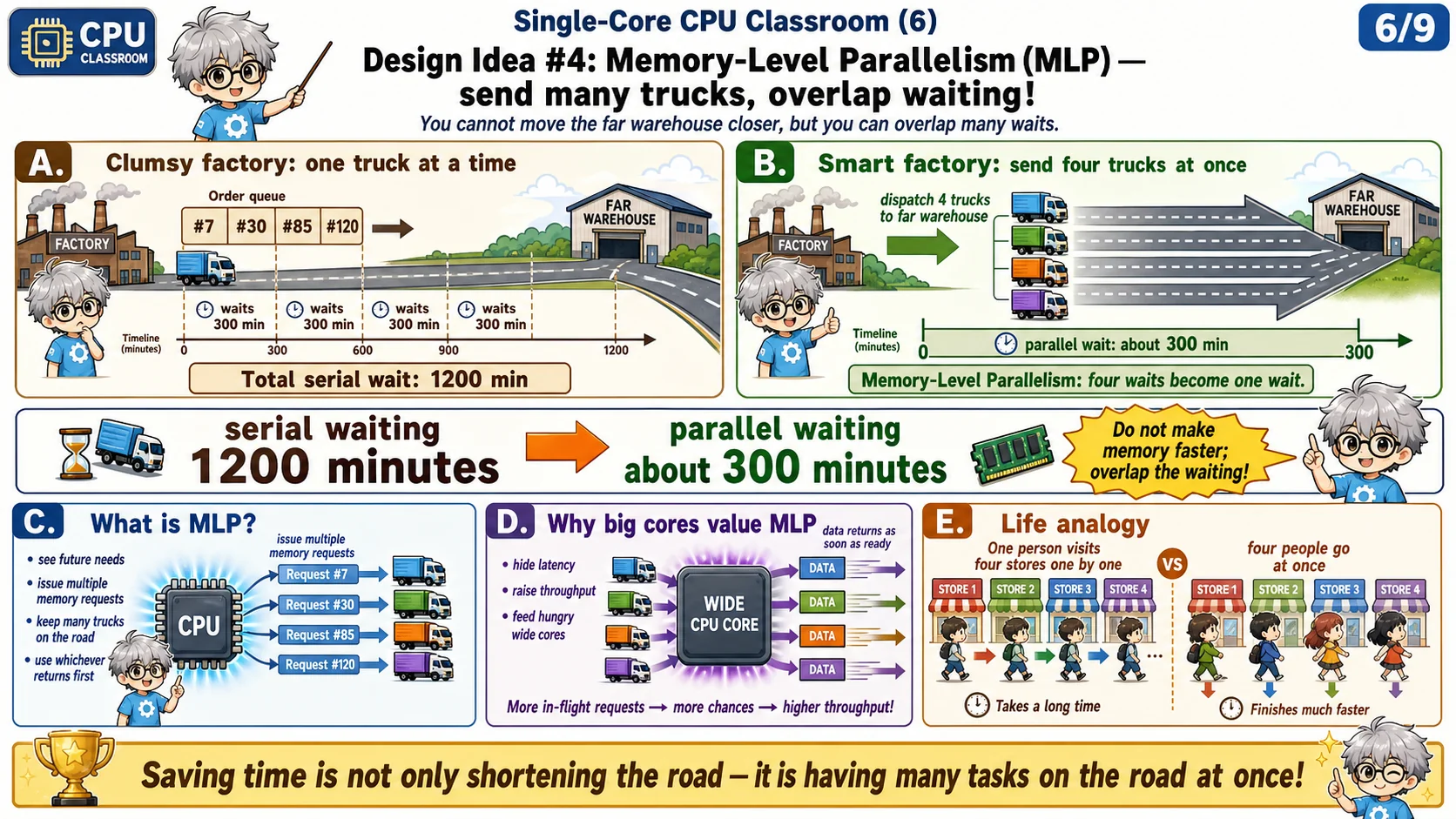
Sometimes the factory needs several deliveries rather than one. A CPU may likewise need several pieces of data that have not arrived. After a cache miss, the request must search the next memory level. A request reaching DRAM may wait hundreds of CPU cycles. The actual latency depends on the platform and load. Waiting for one request at a time puts those delays in sequence.

Use the plate's four trucks to picture overlapping time. Four trips taking 300 minutes each require 1200 minutes if they run serially. Starting together gives an ideal wait of about 300 minutes. Minutes belong to the transport analogy. For the CPU, imagine four reads taking 300 cycles each. Known, independent addresses allow their waits to overlap. Each request remains slow, but the total time may shrink.

This ability is called memory-level parallelism, or MLP. The core must discover several reads early and track unfinished requests. A non-blocking cache can handle other requests while a miss is pending. Miss status holding registers, or MSHRs, track cache blocks that have not returned. The load/store queue and ROB also need free space. The gem5 cache documentation gives an example of non-blocking caches and MSHRs. ^[10]

Four reads cannot always start together. In a linked-list traversal, the next address may come from the previous read's result. MLP then has little opportunity to overlap those reads. Even independent requests can be limited by bandwidth and queue capacity. Four 300-cycle waits are an idealized example, not a promise of fourfold speedup. Diagnose memory bottlenecks by separating single-request latency from the number of requests the system can handle together.

Cache brings data near; prefetch brings it early

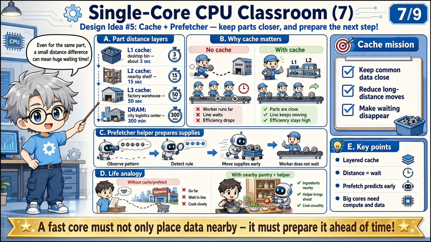
Warehouse placement also affects how long a factory waits. A CPU usually holds data in several memory levels. L1 cache is small and usually has the lowest access latency. L2 is larger and generally slower. Some designs add L3 before DRAM. Distance in the plate represents waiting time, not physical meters. The number of cache levels and whether they are shared depend on the processor design.

Cache exploits locality in program accesses. Recently used data may be needed again soon: temporal locality. An array scan often uses the next nearby element: spatial locality. Cache stores data in blocks, so neighboring elements may arrive together. The program can then avoid some trips to DRAM. Misses still occur when capacity is insufficient or blocks compete for the same cache space.

A prefetcher tries to move data before the program needs it. A sequential array scan often produces a recognizable access pattern. The prefetcher can request later blocks early. If the data arrives in time, subsequent reads spend less time waiting. Irregular accesses are harder to predict. Early or incorrect prefetches consume bandwidth and cache space. They may even evict data that will soon be needed.

The three memory mechanisms have distinct jobs. Cache retains nearby data that may be reused. Prefetching brings likely future data early. MLP overlaps requests that still have to wait. More cache helps when it retains useful data. If our example program keeps waiting for memory, inspect its access pattern and working set first. The working set is the data used during the execution interval. Cache capacity alone cannot predict the size of a speedup.

ISA format affects how easily the frontend feeds the backend

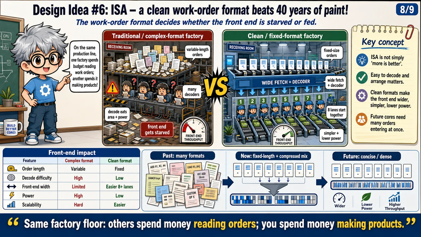
A factory must read its orders as well as receive its materials. A CPU's instruction set architecture, or ISA, defines instruction encodings and the meaning of operations. Registers and memory-access rules are part of that contract. Related architecture specifications also define exceptions and interrupts. Software relies on the contract, and hardware must implement it. Internal scheduling is a microarchitecture choice.

A regular format can simplify some frontend work. Fixed-length instructions, for example, make boundaries easier to locate. Variable lengths require identifying where each instruction starts and ends. Some cores also split instructions into micro-operations. Regularity does not require every instruction to have the same length. RISC-V's C extension allows 16-bit and 32-bit instructions to be mixed. It reduces code size while keeping decoding manageable. The C extension specification describes this trade-off. ^[11]

Code density also affects instruction supply. Expressing the same function in fewer instruction bytes may let the instruction cache hold more work. The meaning of each operation matters too. Vector instructions can process a group of data in one operation. Compiler support affects how effectively a program uses them. Decode difficulty alone therefore cannot rank entire ISAs. A simpler format does not automatically guarantee higher performance.

Compare different ISAs using the completion time for the same job. They may need different instruction counts or split an instruction into different numbers of micro-operations. The processor with higher IPC does not necessarily finish first. The plate's standardized orders help explain frontend cost. They cannot determine which instruction set is fastest. Our computer-selection decision needs the ISA, compiler, and microarchitecture considered under the same test conditions.

Back to the opening question: where did the time go?

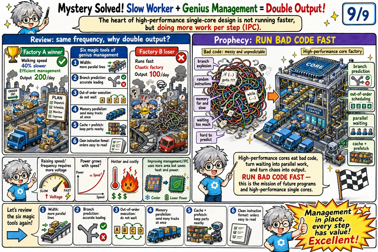
Return to the two computers labeled 3GHz. Equal frequency fixes only the number of cycles per second. If A spends less time waiting, it may finish the job in fewer cycles. The plate's 200 boxes versus 100 boxes per day illustrates different output. It does not claim a twofold advantage for any particular CPU. We still need measurements to establish the difference for our program.

We can now look for where the program waits. If instruction supply is short, examine the frontend and branches. If ready data cannot be processed together, examine dependencies and execution resources. If data is still far away, examine cache misses and overlapping requests. Width provides processing capacity, and out-of-order execution finds ready work. They must cooperate with the supply mechanisms to raise average IPC.

The plate's RUN BAD CODE FAST expresses a design goal. Here, it means programs with frequent branches or irregular accesses. It does not mean the CPU repairs incorrect software or produces the right answer from a broken program. Hardware must still preserve the defined results. Within finite area and power, it tries to reduce waiting. Better software data layouts or dependency chains may also help the hardware work effectively.

Change one condition: our program now reads a linked list one node at a time. Does a wider pipeline guarantee improvement? No. The next address arrives with the current node's data, so independent work may be scarce. MLP is limited too. This lesson leaves vector execution, TLB address translation, and operating-system scheduling for deeper study. The multicore sequel asks a related question: after adding cores, which parts of the job must still wait in line?

References

1. SPEC CPU 2017 Overview: Benchmarking context for CPU speed and rate measurements.
2. SPEC CPU 2017 Run and Reporting Rules: Additional context for interpreting speed and rate results.
3. gem5 O3CPU Documentation: Reference model for out-of-order execution, ROB, execute-in-execute, and commit behavior.
4. gem5 Memory System Documentation: Background on cache hierarchy and memory request modeling.
5. Linux Kernel Documentation: Cache and TLB Flushing: Operating-system view of cache and TLB behavior.
6. Linux Kernel Documentation: Memory Management Concepts: Memory hierarchy and address-translation background.
7. RISC-V ISA Manual Releases: Official release location for RISC-V ISA specifications and instruction-format context.
8. Agner Fog: The Microarchitecture of Intel, AMD and VIA CPUs: Practical microarchitecture reference covering decoding, branch prediction, out-of-order execution, and cache behavior.
9. Hennessy and Patterson, Computer Architecture: A Quantitative Approach: Classic architecture textbook reference for quantitative performance, ILP, and memory hierarchy.
10. gem5 Classic Caches: Model of non-blocking caches, MSHRs, and outstanding requests.
11. RISC-V C Extension, Version 2.0: Rules for mixing 16-bit compressed and 32-bit instructions.